Getting started

To start your experience with SPOTPY you need to have SPOTPY installed. Please see the Installation chapter for further details.

You will find the following example in the getting_started.py file under the folder /examples. There is no need for copy paste work.

To use SPOTPY we have to import it and use one of the pre-build examples:

import spotpy                                                # Load the SPOT package into your working storage 
from spotpy import analyser                                  # Load the Plotting extension 
from spotpy.examples.spot_setup_rosenbrock import spot_setup # Import the two dimensional Rosenbrock example

The example comes along with parameter boundaries, the Rosenbrock function, the optimal value of the function and RMSE as a objective function. So we can directly start to analyse the Rosenbrock function with one of the algorithms. We start with a simple Monte Carlo sampling:

# Give Monte Carlo algorithm the example setup and saves results in a RosenMC.csv file
sampler = spotpy.algorithms.mc(spot_setup(), dbname='RosenMC', dbformat='csv')

Now we can sample with the implemented Monte Carlo algorithm:

sampler.sample(100000)                # Sample 100.000 parameter combinations
results=sampler.getdata()             # Get the results of the sampler

Now we want to have a look at the results. First we want to know, what the algorithm has done during the 100.000 iterations:

spotpy.analyser.plot_parameterInteraction(results)     # Use the analyser to show the parameter interaction

This should give you a parameter interaction plot of your results, which should look like Fig. 1:

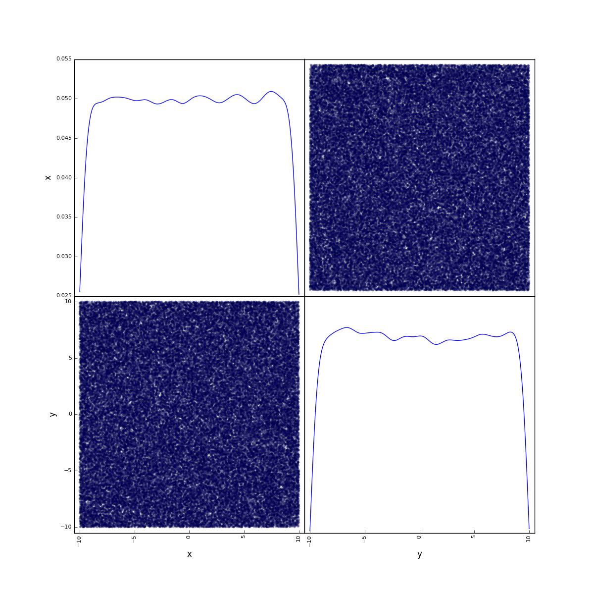
Figure 1: Parameter interaction of the two dimensional Rosenbrock function

We can see that the parameters x and y, which drive the the Rosenbrock function, vary between -10 and 10.

If you want to see the best 10% of your samples, which is called posterior parameter distribution, you have to do something like this:

posterior=spotpy.analyser.get_posterior(results, percentage=10)
spotpy.analyser.plot_parameterInteraction(posterior)

This should give you a parameter interaction plot of your best 10% samples, which should look like Fig. 2:

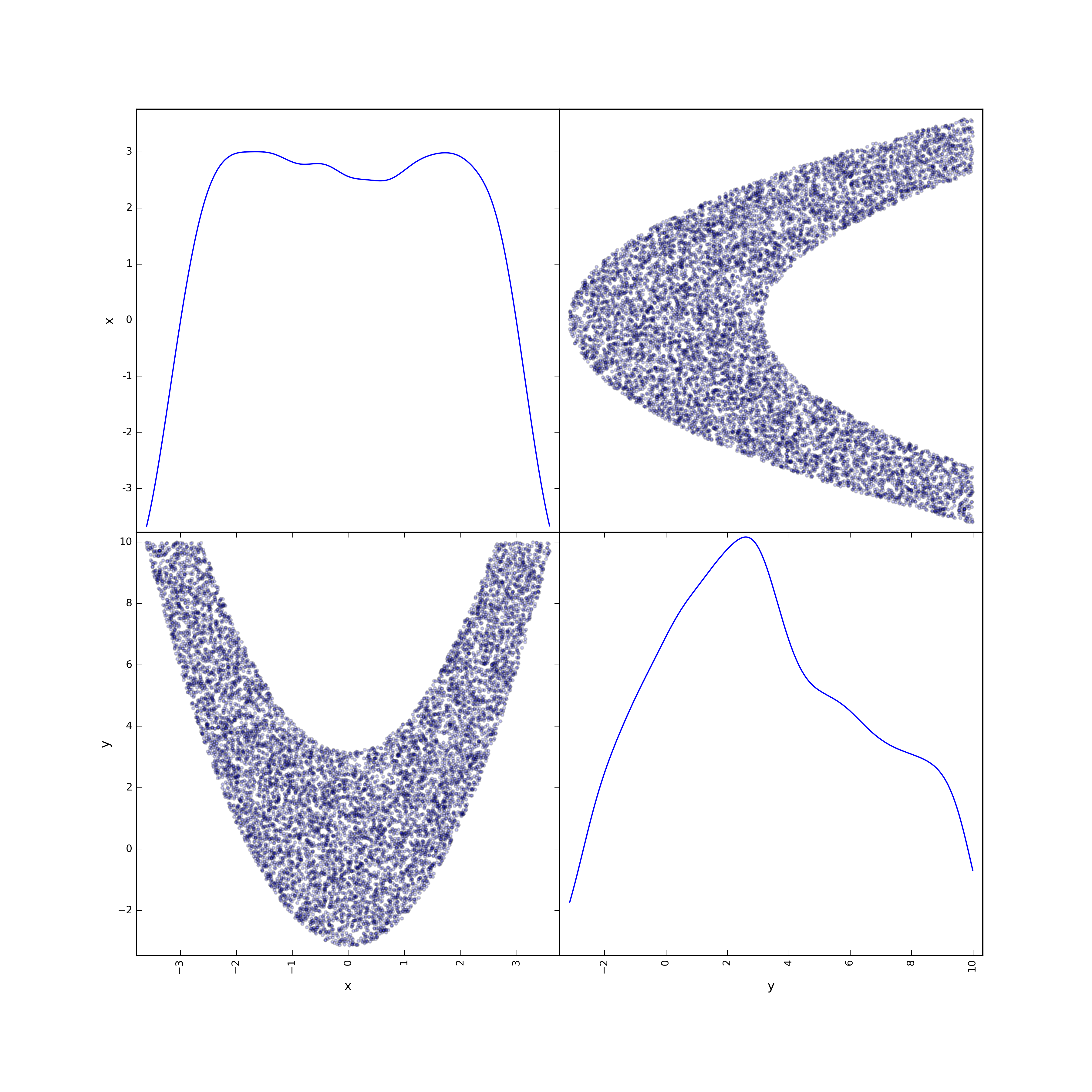
Figure 2: Posterior parameter interaction of the two dimensional Rosenbrock function

This has reduced your parameter uncertainty for x of around 70% and for y for 40%, which is telling us, that we have a higher uncertainty for y than for x in our Rosenbrock example.

Note that your results are a normal NumPy array. That means you are not limited to pre-build plotting features and you can try out things on your own, e.g. like typing plot(results['like']).

Let us find out the best found parameter set:

print(spotpy.analyser.get_best_parameterset(results))

And you will get something like

>>> x=1.05  y=1.12

depending on your random results. The optimal best values for the Rosenbrock function are x=1 and y=1.

Check out chapter Rosenbrock Tutorial to see how the Rosenbrock function really looks like.