Calibration of HYMOD with SCE-UA

This chapter shows you, how to calibrate an external hydrological model (HYMOD) with SPOTPY.

We use the previously created hydrological model HYMOD spotpy_setup class as an example, to perform a calibration with the Shuffled Complex Evolution Algorithm (SCE-UA) algorithm. For detailed information about the underlying theory, have a look at Duan, Q., Sorooshian, S. and Gupta, V. K. (1994) Optimal use of the SCE-UA global optimization method for calibrating watershed models, J. Hydrol..

First some relevant functions are imported Hymod example:

import numpy as np
import spotpy
from spotpy.examples.spot_setup_hymod_python import spot_setup
import matplotlib.pyplot as plt

As SCE-UA is minizing the objective function we need a objective function that gets better with decreasing values. The Root Mean Squared Error objective function is a suitable choice:

spot_setup=spot_setup(spotpy.objectivefunctions.rmse)

Now we create a sampler, by using one of the implemented algorithms in SPOTPY. The algorithm needs the inititalized spotpy setup class, and wants you to define a database name and database format. Here we create a SCEUA_hymod.csv file, which will contain the returned likelihood function, the coresponding parameter set, the model results and a chain ID (SCE-UA is starting different independent optimization complexes, which need to be in line, to receive robust results, they are herein called chains):

sampler=spotpy.algorithms.sceua(spot_setup, dbname='SCEUA_hymod', dbformat='csv')

To actually start the algorithm, spotpy needs some further details, like the maximum allowed number of repetitions, the number of chains used by dream (default = 5) and set the Gelman-Rubin convergence limit (default 1.2). We further allow 100 runs after convergence is achieved:

#Select number of maximum repetitions
rep=5000

We start the sampler and set some optional algorithm specific settings (check out the publication of SCE-UA for details):

sampler.sample(rep, ngs=7, kstop=3, peps=0.1, pcento=0.1)

Access the results

All gained results can be accessed from the SPOTPY csv-database:

results = spotpy.analyser.load_csv_results('SCEUA_hymod')

These results are stored in a simple structered numpy array, giving you all the flexibility at hand to analyse the results. Herein we show a example how the objective function was minimized during sampling:

fig= plt.figure(1,figsize=(9,5))
plt.plot(results['like1'])
plt.show()
plt.ylabel('RMSE')
plt.xlabel('Iteration')
fig.savefig('SCEUA_objectivefunctiontrace.png',dpi=300)

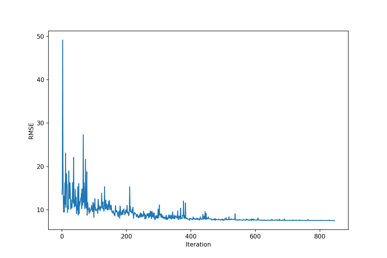Figure 1: Root Mean Squared Error of Hymod model results during the optimization with SCE-UA algorithm.

Plot best model run

Or if you want to check the best model run, we first need to find the run_id with the minimal objective function value

bestindex,bestobjf = spotpy.analyser.get_minlikeindex(results)

Than we select the best model run:

best_model_run = results[bestindex]

And filter results for simulation results only:

fields=[word for word in best_model_run.dtype.names if word.startswith('sim')]
best_simulation = list(best_model_run[fields])

The best model run can be plotted by using basic Matplotlib skills:

fig= plt.figure(figsize=(16,9))
ax = plt.subplot(1,1,1)
ax.plot(best_simulation,color='black',linestyle='solid', label='Best objf.='+str(bestobjf))
ax.plot(spot_setup.evaluation(),'r.',markersize=3, label='Observation data')
plt.xlabel('Number of Observation Points')
plt.ylabel ('Discharge [l s-1]')
plt.legend(loc='upper right')
fig.savefig('SCEUA_best_modelrun.png',dpi=300)

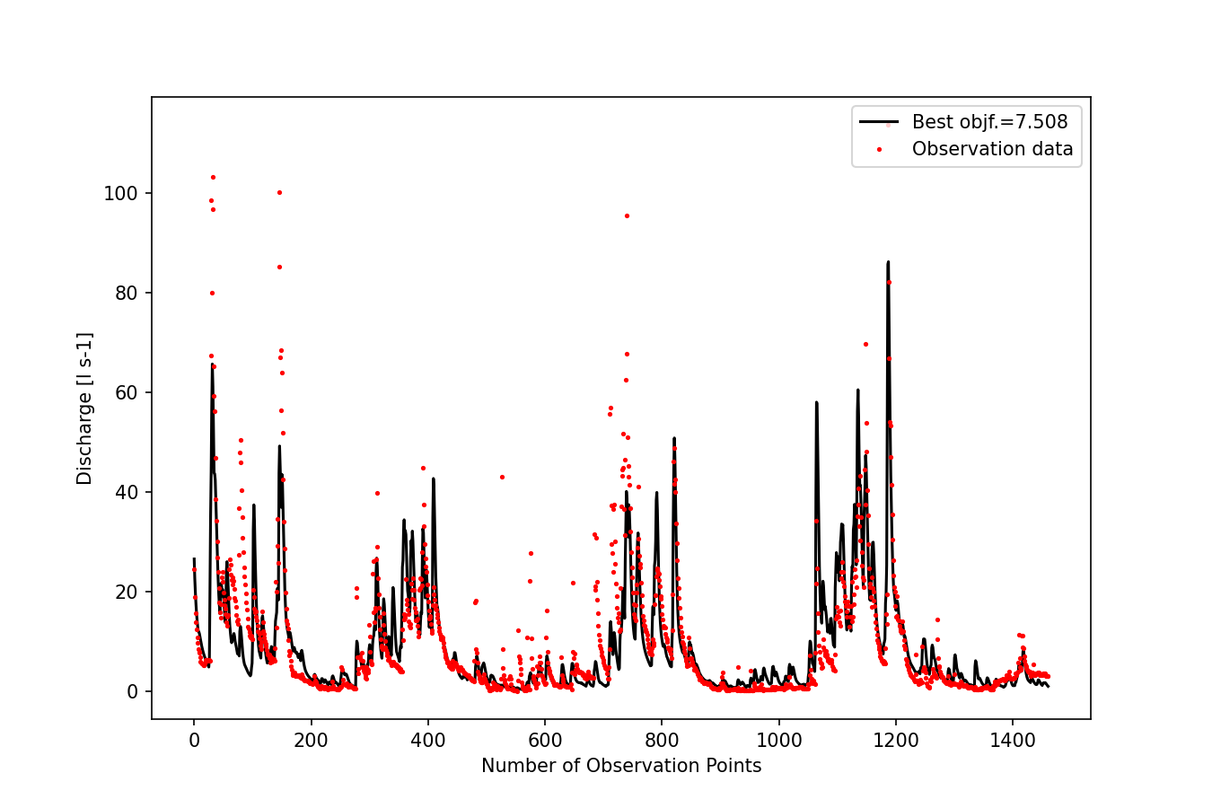
Figure 2: Best model run of HYMOD, calibrated with SCE-UA, using RMSE as objective function.

The corresponding code is available for download here.