The Ackley
The Ackley function is another challenging optimization problem. With just one small global optimum. It is defined as:
$$f_{Ackley}(x_0 \cdots x_n) = -20 exp(-0.2 \sqrt{\frac{1}{n} \sum_{i=1}^n x_i^2}) - exp(\frac{1}{n} \sum_{i=1}^n cos(2\pi x_i)) + 20 + e$$
where the control variables are -32.768 < x_i < 32.768, with f(x_i=0) = 0.
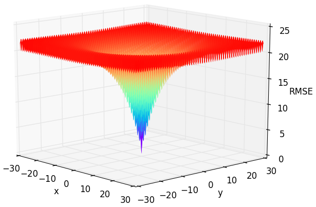
Figure 4: Response surface of the two dimensional Ackley function. Check out /examples/3dplot.pyto produce such plots.
Creating the setup file
This time we want to challenge our algorithms with a high number of dimensions. We use the __init__ function to create 50 parameters.
We give every parameter just a number and not a name. See /examples/spotpy_setup_ackley.py for the following code:
class spotpy_setup(object):
    def __init__(self,dim=30):
        self.dim=dim
        self.params = []
        for i in range(self.dim):
            self.params.append(spotpy.parameter.Uniform(str(i),-32.768,32.768,2.5,-20.0))

    def parameters(self):
        return spotpy.parameter.generate(self.params)

    def simulation(self, vector):
        firstSum = 0.0
        secondSum = 0.0
        for c in vector:
            firstSum += c**2.0
            secondSum += np.cos(2.0*np.pi*c)
            n = float(len(vector))
        return [-20.0*np.exp(-0.2*np.sqrt(firstSum/n)) - np.exp(secondSum/n) + 20 + np.e]

    def evaluation(self):
        observations=[0]
        return observations

    def objectivefunction(self,simulation,evaluation):
        objectivefunction= -spotpy.objectivefunctions.rmse(evaluation,simulation)
        return objectivefunction
Sampling
Now that we crated our setup file, we want to start to investigate our function. One way is to analyse the results of the sampling is to have a look at the objective function trace of the sampled parameters.
We start directly with all algorithms. First we have to create a new file:
import spotpy
from spotpy.examples.spotpy_setup_ackley import spotpy_setup   # Load your just created file from above
Now we create samplers for every algorithm and Now sample 25,000 parameter combinations for every algorithm
spotpy_setup=spotpy_setup()
sampler=spotpy.algorithms.mc(spotpy_setup,    dbname='ackleyMC',    dbformat='csv')
sampler.sample(rep)
results.append(sampler.getdata())

sampler=spotpy.algorithms.lhs(spotpy_setup,   dbname='ackleyLHS',   dbformat='csv')
sampler.sample(rep)
results.append(sampler.getdata())

sampler=spotpy.algorithms.mle(spotpy_setup,   dbname='ackleyMLE',   dbformat='csv')
sampler.sample(rep)
results.append(sampler.getdata())

sampler=spotpy.algorithms.mcmc(spotpy_setup,  dbname='ackleyMCMC',  dbformat='csv')
sampler.sample(rep)
results.append(sampler.getdata())

sampler=spotpy.algorithms.sceua(spotpy_setup, dbname='ackleySCEUA', dbformat='csv')
sampler.sample(rep,ngs=2)
results.append(sampler.getdata())

sampler=spotpy.algorithms.sa(spotpy_setup,    dbname='ackleySA',    dbformat='csv')
sampler.sample(rep)
results.append(sampler.getdata())

sampler=spotpy.algorithms.demcz(spotpy_setup, dbname='ackleyDEMCz', dbformat='csv')
sampler.sample(rep,nChains=30)
results.append(sampler.getdata())

sampler=spotpy.algorithms.rope(spotpy_setup,  dbname='ackleyROPE',  dbformat='csv')
sampler.sample(rep)
results.append(sampler.getdata())
Plotting
To plot our results, we need just a few lines of code:
algorithms=['MC','LHS','MLE','MCMC','SCEUA','SA','DEMCz','ROPE']
evaluation = spotpy_setup.evaluation()
spotpy.analyser.plot_likelihoodtraces(results,evaluation,algorithms)
This should give you something like this:
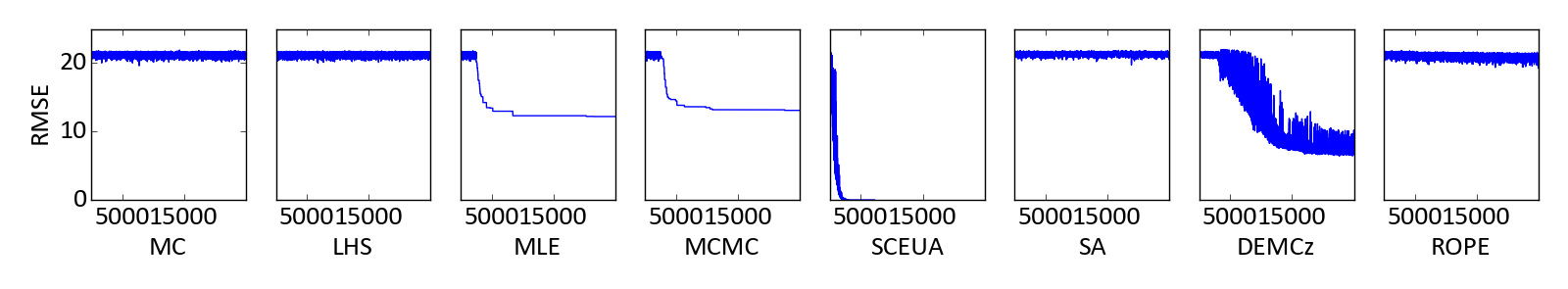
Figure 5: Objective function trace of 30 dimensional Ackley function.