Bayesian uncertainty analysis of HYMOD with DREAM

This chapter shows you, how to calibrate an external hydrological model (HYMOD) with SPOTPY.

We use the previously created hydrological model HYMOD spotpy_setup class as an example, to perform a parameter uncertainty analysis and Bayesian calibration with the Differential Evolution Adaptive Metropolis (DREAM) algorithm. For detailed information about the underlying theory, have a look at the Vrugt (2016).

First some relevant functions are imported Hymod example:

import numpy as np
import spotpy
import matplotlib.pyplot as plt
from spotpy.likelihoods import gaussianLikelihoodMeasErrorOut as GausianLike
from spotpy.analyser import plot_parameter_trace
from spotpy.analyser import plot_posterior_parameter_histogram

Further we need the spotpy_setup class, which links the model to spotpy:

from spotpy.examples.spot_setup_hymod_python import spot_setup

It is important that this function is initialized before it is further used by SPOTPY:

spot_setup=spot_setup()

In this special case, we want to change the implemented rmse objective function with a likelihood function, which is compatible with the Bayesian calibration approach, used by the DREAM sampler:

# Initialize the Hymod example (will only work on Windows systems)
spot_setup=spot_setup(GausianLike)

Sample with DREAM

Now we create a sampler, by using one of the implemented algorithms in SPOTPY. The algorithm needs the inititalized spotpy setup class, and wants you to define a database name and database format. Here we create a DREAM_hymod.csv file, which will contain the returned likelihood function, the coresponding parameter set, the model results and a chain ID (Dream is starting different independent optimization chains, which need to be in line, to receive robust results):

sampler=spotpy.algorithms.dream(spot_setup, dbname='DREAM_hymod', dbformat='csv')

To actually start the algorithm, spotpy needs some further details, like the maximum allowed number of repetitions, the number of chains used by dream (default = 5) and set the Gelman-Rubin convergence limit (default 1.2). We further allow 100 runs after convergence is achieved:

#Select number of maximum repetitions
rep=5000

# Select five chains and set the Gelman-Rubin convergence limit
nChains                = 4
convergence_limit      = 1.2

# Other possible settings to modify the DREAM algorithm, for details see Vrugt (2016)
nCr                    = 3
eps                    = 10e-6
runs_after_convergence = 100
acceptance_test_option = 6

We start the sampler and collect the gained r_hat convergence values after the sampling:

r_hat = sampler.sample(rep, nChains, nCr, eps, convergence_limit)

Access the results

All gained results can be accessed from the SPOTPY csv-database:

results = spotpy.analyser.load_csv_results('DREAM_hymod')

These results are structured as a numpy array. Accordingly, you can access the different columns by using simple Python code, e.g. to access all the simulations:

fields=[word for word in results.dtype.names if word.startswith('sim')]
print(results[fields)

Plot model uncertainty

For the analysis we provide some examples how to plor the data. If you want to see the remaining posterior model uncertainty:

fig= plt.figure(figsize=(16,9))
ax = plt.subplot(1,1,1)
q5,q25,q75,q95=[],[],[],[]
for field in fields:
    q5.append(np.percentile(results[field][-100:-1],2.5))
    q95.append(np.percentile(results[field][-100:-1],97.5))
ax.plot(q5,color='dimgrey',linestyle='solid')
ax.plot(q95,color='dimgrey',linestyle='solid')
ax.fill_between(np.arange(0,len(q5),1),list(q5),list(q95),facecolor='dimgrey',zorder=0,
                linewidth=0,label='parameter uncertainty')  
ax.plot(spot_setup.evaluation(),'r.',label='data')
ax.set_ylim(-50,450)
ax.set_xlim(0,729)
ax.legend()
fig.savefig('python_hymod.png',dpi=300)

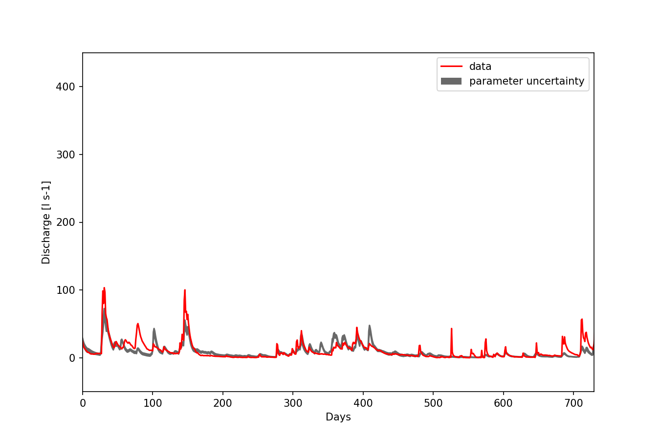Figure 1: Posterior model uncertainty of HYMOD.

Plot convergence diagnostic

If you want to check the convergence of the DREAM algorithm:

spotpy.analyser.plot_gelman_rubin(results, r_hat, fig_name='python_hymod_convergence.png')

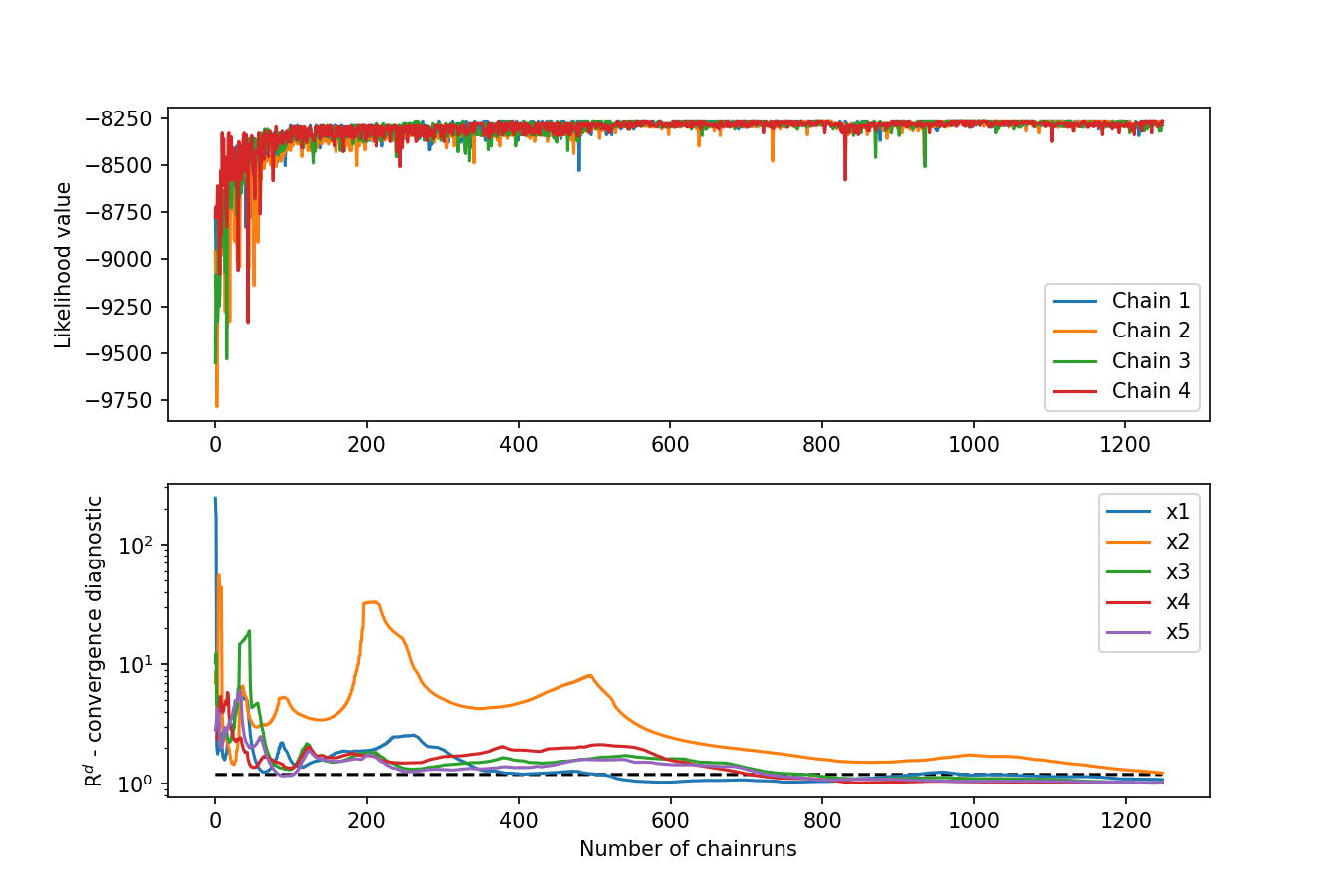
Figure 2: Gelman-Rubin onvergence diagnostic of DREAM results.

Plot parameter uncertainty

Or if you want to check the posterior parameter distribution:

parameters = spotpy.parameter.get_parameters_array(spot_setup)

fig, ax = plt.subplots(nrows=5, ncols=2)
for par_id in range(len(parameters)):
    plot_parameter_trace(ax[par_id][0], results, parameters[par_id])
    plot_posterior_parameter_histogram(ax[par_id][1], results, parameters[par_id])

ax[-1][0].set_xlabel('Iterations')
ax[-1][1].set_xlabel('Parameter range')

plt.show()
fig.savefig('hymod_parameters.png',dpi=300)

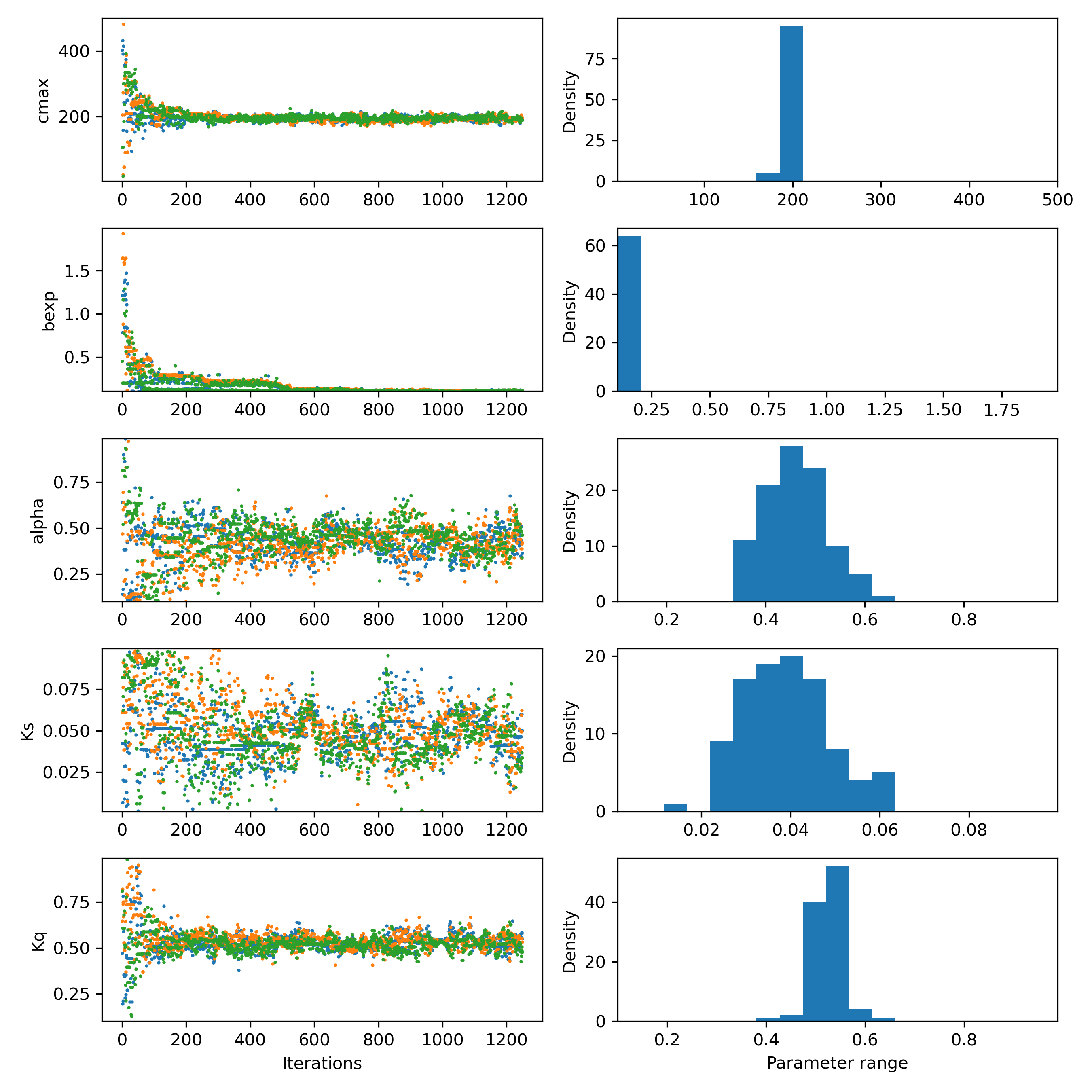
Figure 3: Posterior parameter distribution of HYMOD. Plotting the last 100 repetitions of the algorithm as a histogram.

The corresponding code is available for download here.