Algorithm Guide
SPOTPY comes along with some very powerful techniques for parameter optimization. The conducted algorithms can be very efficient, but also inefficient, depending on your specific parameter search problem. This is why we have developed a decision tree to help you choosing the right algorithm:
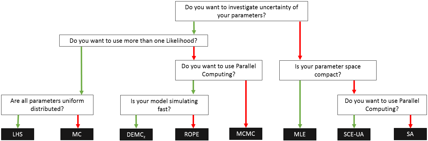
Figure 8: Decision-tree as a guidance for the choice of an algorithm in SPOTPY for a specific optimization problem.
Algorithm Overview
To understand, what the algorithms are doing, we can provide a short overview.
MC
Monte Carlo
This algorithm is probably the simplest one. It relays on repeated random parameter samplings which are tested in the simulation function. The algorithm does not learn or adopt its method during the sampling, which makes it easy to parallelize. In principle, this algorithm can solve any parameter search problem, but with an increasing number of parameters, the number of needed iterations is rising exponential. This can be optimized by selecting an appropriate distribution for the parameters.
These steps are performed during the sampling:
- Create random parameter set
- Run simulation function with the parameter set
- Compare resulting simulation with evaluation values and calculate a objective function
- Save objective function, parameter set and simulation in a database
Because of its simplicity and easy integration the Monte Carlo sampling is widely used.
LHS
Latin Hypercube Sampling
The Latin Hypercube sampling combines the dimensions of the parameter function with the number of iterations into one matrix. This matrix assures that every parameter combination is scanned. The needed number of iterations (N_{max}) can be calculated with the following formula:
$$N_{max} = (k!)^{p-1}$$
with k as divisions per parameter and p as number of parameters.
These steps are performed during the sampling:
- Check the minimal and maximal value of every parameter
- Create the Latin HyperCube matrix
- Run simulation function with every row of the matrix
- Save every objective function, parameter set and simulation in a database
For further detailed information check out McKay et al. (1979).
MCMC
Markov Chain Monte Carlo
The famous Metropolis MCMC is one of the most used parameter optimization method. It can learn during the sampling and can deal with non-monotonically response functions. The sampling method can reject regions of the parameter search space and tries to find the global optimum. The more often a region of the parameter search space was sampled, the more likely it is to be the global optimum.
These steps are performed during the sampling:
- 10% of the repetitions are designed to perform a Monte Carlo sampling (burn-in period)
- Save likelihood, parameter set and simulation in a database
- The best parameter set is taking after the burn-in as an inital parameter set for the Metropolis sampler
- A random value with a Gaussian distribution around the last best found parameter set is drawn to generate a new parameter-set (mean= last best parameter set, standard deviation=step-size of parameters function)
- Run simulation function with the new parameter set
- Calculate a user defined likelihood function
- Decide if the new parameter is accepted through a Metropolis decision
- Save the last accepted run with likelihood, parameter set and simulation in a database
The MCMC algorithm can find a (quasi-) global optimum, but with a still remaining risk to stuck in local minima, depending on the chosen step-size in the parameter function. Is the step-size to large, the sampler jumps too often away from the optimum. Is the step size to low, it can get stuck in local minima.
For further detailed information check out Metropolis et al. (1953).
MLE
Maximum Likelihood Estimation
If one is just interested in a fast calibration of a simple model (with nearly monotonically response function or a compact parameter search space), the MLE is an efficient choice. To test whether the MLE algorithm is applicable for calibrating the desired model, it is recommend to test the model with MC first. MLE maximizes the likelihood during the sampling, by adapting the parameter only in directions with an increasing likelihood.
These steps are performed during the sampling:
- 10% of the repetitions are designed to perform a Monte Carlo sampling (burn-in period)
- Save likelihood, parameter set and simulation in a database
- The best parameter set is taking after the burn-in as an initial parameter set for the Metropolis sampler
- A random value with a Gaussian distribution around the last best found parameter set is drawn to generate a new parameter-set (mean= last best parameter set, standard deviation=step-size of parameters function)
- Run simulation function with the new parameter set
- Compare resulting simulation with evaluation values and calculate a likelihood
- Accept new parameter if it is better than the so far best found parameter set
- Save the best run with likelihood, parameter set and simulation in a database
Adopted in the right way, the MLE can be a very efficient algorithm. But the risk to stuck in local optima is high.
SA
Simulated Annealing
Simulated Annealing can be a robust algorithm, but needs to be adopted to every new parameter search problem. The algorithm starts with a high chance to jump to a new point (high temperature), which is getting more and more unlikely with increasing repetitions (cooling down). If everything works, the algorithm freezes at the global optimal parameter-set.
- The optimal-guess parameter set is taking as an initial parameter set for Simulated Annealing
- Run simulation function with the new parameter set
- Compare resulting simulation with evaluation values and calculate a objective function
- Save objectivefunction, parameter set and simulation in a database
- Generated a new parameter set
- Run simulation function with the new parameter set
- Accept new objective function if its better than the last best found, or, if worse, accept new objective function with Boltzmann distribution, depending on the temperature of the system
- Save the last accepted run with objective function, parameter set and simulation in a database
For further detailed information check out Kirkpatrick et al. (1985).
ROPE
RObust Parameter Estimation
Another non-Bayesian approach is the ROPE algorithm. It determines parameter uncertainty with the concept of data depth. This has the benefit, that the resulting parameter sets have proven to be more likely giving good results when space or time period of the model changes, e.g. for validation.
- 25% of the repetitions are designed to perform a Monte Carlo sampling (burn-in period)
- The best 10% of the results are taken to generate samples (another 25% of the repetitions) in the remaining multi-dimensional parameter space.
- Run simulation function with generated parameter sets
- Save every objective function, parameter set and simulation in a database
- The best 10% of the results are taken to generate samples (another 25% of the repetitions) in the remaining multi-dimensional parameter space.
- Run simulation function with generated parameter sets
- Save every objective function, parameter set and simulation in a database
- The best 10% of the results are taken to generate samples (another 25% of the repetitions) in the remaining multi-dimensional parameter space.
- Run simulation function with generated parameter sets
- Save every objective function, parameter set and simulation in a database
For further detailed information check out Bardossy et al. (2008).
SCE-UA
Shuffled Complex Evolution - University of Arizona
SCE-UA is designed to overcome the risk of MCMC to stuck in local optima. The risk was reduced by starting several chains/complexes that evolve individually in the parameter space. The population is periodically shuffled and new complexes are created with information from the previous complex. SCE-UA has found to be very robust in finding the global optimum of hydrological models and is one the most widely used algorithm in hydrological applications today.
- 10% of the repetitions are designed to perform a Monte Carlo sampling (burn-in period)
- Generate a complex and evolve each complex independent by taking evolution steps
- Run simulation function with generated parameter sets
- Calculate a hardcoded RootMeanSquaredError (RMSE) as objective function
- Save every objective function, parameter set and simulation in a database
- Check convergence, if criterion is reached, stop
- Shuffle complexes: Combine complexes and sort the objective functions
- Check complex number reduction
- Generate a new complex
For further detailed information check out Duan et al. (1994).
DE-MCz
Differential Evolution Markov Chain
One of the most recent algorithms we present here is the DE MCz. It requires a minimal number of three chains that learn from each other during the sampling. It has the same Metropolis decision as the MCMC algorithm and has found to be quite efficient compared with other MCMC techniques. Like SCE-UA and SA, DE-MCz does not require any prior distribution information, which reduces the uncertainty due to subjective assumptions during the analysis.
- Initialize matrix by sampling from the prior
- Sample uniformly for all chains
- Generate a new parameter set
- Run simulation function with generated parameter sets
- Calculate a user defined likelihood function
- Decide if the new parameter is accepted through a Metropolis decision
- Check convergence, if criterion is reached, stop
For further detailed information check out terBraak et al. (2008).