The Griewank
The Griewank function is known to be a challenge for parameter estimation methods. It is defined as:
$$f_{Griewank}(x,y) = \frac{x²+y²}{4000}-cos(\frac{x}{\sqrt{2}})cos(\frac{y}{\sqrt{3}})+1$$
where the control variables are -50 < x < 50 and -50 < y < 50, with f(x=0,y=0) = 0.
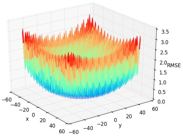
Figure 2: Response surface of the two dimensional Griewank function. Check out /examples/3dplot.pyto produce such plots.
Creating the setup file
This time we create a more general model setup. We use the __init__ function to set the number of parameters we want to analyse.
In this case we select two parameters. See /examples/spotpy_setup_griewank.py for the following code:
import numpy as np
import spotpy

class spotpy_setup(object):
    def __init__(self):
        self.dim=2
        self.parameternames=['x','y']
        self.params=[]
        for parname in self.parameternames:
            spotpy.parameter.Uniform(parname,-10,10,1.5,3.0)

    def parameters(self):
        return spotpy.parameter.generate(self.params)

    def simulation(self, vector):
        n = len(vector)
        fr = 4000
        s = 0
        p = 1
        for j in range(n):
            s = s+vector[j]**2
        for j in range(n):
            p = p*np.cos(vector[j]/np.sqrt(j+1))
        simulation = [s/fr-p+1]
        return simulation

    def evaluation(self):
        observations=[0]
        return observations

    def objectivefunction(self,simulation,evaluation):
        objectivefunction= -spotpy.objectivefunctions.rmse(evaluation,simulation)
        return objectivefunction
Sampling
Now that we crated our setup file, we want to start to investigate our function. One way is to analyse the results of the sampling is to have a look at the objective function trace of the sampled parameters.
We start directly with all algorithms. First we have to create a new file:
import spotpy
from spotpy_setup_griewank import spotpy_setup   # Load your just created file from above
Now we create samplers for every algorithm and sample 5,000 parameter combinations for every algorithm:
results=[]
spotpy_setup=spotpy_setup()
rep=5000

sampler=spotpy.algorithms.mc(spotpy_setup,    dbname='GriewankMC',    dbformat='csv')
sampler.sample(rep)
results.append(sampler.getdata())

sampler=spotpy.algorithms.lhs(spotpy_setup,   dbname='GriewankLHS',   dbformat='csv')
sampler.sample(rep)
results.append(sampler.getdata())

sampler=spotpy.algorithms.mle(spotpy_setup,   dbname='GriewankMLE',   dbformat='csv')
sampler.sample(rep)
results.append(sampler.getdata())

sampler=spotpy.algorithms.mcmc(spotpy_setup,  dbname='GriewankMCMC',  dbformat='csv')
sampler.sample(rep)
results.append(sampler.getdata())

sampler=spotpy.algorithms.sceua(spotpy_setup, dbname='GriewankSCEUA', dbformat='csv')
sampler.sample(rep)
results.append(sampler.getdata())

sampler=spotpy.algorithms.sa(spotpy_setup,    dbname='GriewankSA',    dbformat='csv')
sampler.sample(rep)
results.append(sampler.getdata())

sampler=spotpy.algorithms.demcz(spotpy_setup, dbname='GriewankDEMCz', dbformat='csv')
sampler.sample(rep)
results.append(sampler.getdata())

sampler=spotpy.algorithms.rope(spotpy_setup,  dbname='GriewankROPE',  dbformat='csv')
sampler.sample(rep)
results.append(sampler.getdata())
Plotting
To compare the results of the different algorithms, we choose to show our sampled parameter combinations over a heat map of the Griewank function. This makes it easier to see, whether the algorithms find the local minima or not:
algorithms=['MC','LHS','MLE','MCMC','SCEUA','SA','DEMCz','ROPE']
spotpy.analyser.plot_heatmap_griewank(results,algorithms)
This should give you something like this:
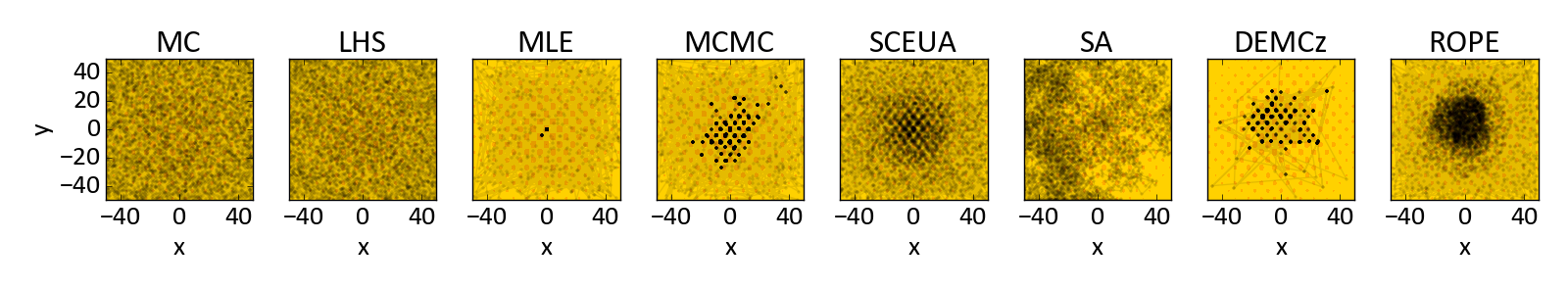
Figure 3: Heat map of the two dimensional Griewank function.